So, you’ve found an error and now you need to figure out what the issue is and hopefully correct it. There are plenty of pages that address specific error types; if you’re looking for one of those, look here (TBA). This article is more about the process of troubleshooting than the trouble itself.
Generally, with Excel you’ll have one of two types of problems:
a) The formula isn’t working
b) The formula is “working”
In both options, the process for troubleshooting is quite straightforward but often full of steps that require careful reading and/or testing of your previous work.
Option ‘a’ generally involves an error value (eg. #VALUE!, #N/A, #NAME?, etc) and no actual value returned. Option ‘b’ is often when things appear to be working but the output isn’t what you expected it to be.
- Is my problem type ‘a’ or ‘b’?
- Is my output an error?
- Does my output make sense?
This is really the first question we need to ask because it forms the basis of our understanding when searching for the issue.
After answering that first one, let’s continue with questions you’d ask for both, and how you might answer them. Now, these might seem straight forward and like common sense – that’s because they are. Occam’s razor and anecdotal evidence all support looking for the most obvious and simple answers first.
- Is my problem type ‘a’ or ‘b’? (as above)
- Does my formula have any obvious errors?
- Are any of my formula arguments1 appearing as an # error? (Relates to Q3)
- Can Excel answer the question I’m asking?
- Does the sheet I’m referencing exist? (Q2)
- Does the table I’m referencing exist? (Q2)
- Does the cell I’m referencing have data?
- Is that data the right data type (most relevant when comparing or searching for values)
- Does the cell I’m referencing have the data I expect?
These are the most obvious answers that are often the cause of simple errors, particularly in shared workbooks, lets walk through them.
Q2. Does my formula have any obvious errors?
Consider the formula below.
=VLOOKUP(D2, A1:B5, 2, FALSE)That formula contains no errors. An error might look like the snippet below;
=VLOOKUP(#REF!, A1:B5, 2, FALSE)This indicates that the item you were referring to has been renamed, moved, or deleted.
Fixing this is often as simple as finding what argument should be there and either adding a new argument that will correct the error or returning the missing data to where it should be. In the above example, we need to find what value this VLOOKUP is meant to be finding in the range defined in the function.
Often when you delete a cell or modify a column/row, Excel will be smart enough to figure some of it out.
Looking at the below example:
Fig 1. shows the working formula, i.e. there are no errors in the formula, and we have the result that we want and expect.
=VLOOKUP(D2, A1:B5, 2, FALSE)
Fig 2. shows it ‘working’, i.e. there are no errors in the formula, and we have exactly the result that we’ve asked for but NOT the result we were expecting.
By ‘working’ I mean that there are no errors in the formula and it’s attempting to do exactly what you’re asking it to but that there can be no result. Read on to see why that’s the case.
=VLOOKUP(C2, A1:A5, 2, FALSE)
Q2 Answer: No, your formula contains no obvious errors.
Q3. Can Excel answer the question I’m asking?
Does the sheet I’m referencing exist? Yes, I only have one sheet.
Does the table I’m referencing exist? Yes, my table exists at A1:A5
Does the cell I’m referencing have data? Yes.
C2 = 3
A1:A5 = numbers
column index 2 = …..
And there’s our problem.
You’ll notice that in Fig 2, there are no errors in the formula as the search value reference has updated from D2 to C2 meaning that Excel still know where to look for the search value. It has also updated the search range to be A1:A5 so it’s searching in the remaining column. It hasn’t, however, been able to modify the column index number, which is still 2.
The formula is effectively trying to return a value that doesn’t exist because the count of columns is 1 but our column index is 2. Due to this error the function returns a #REF! error.
Great news – we’ve found our error! Let’s try another one.
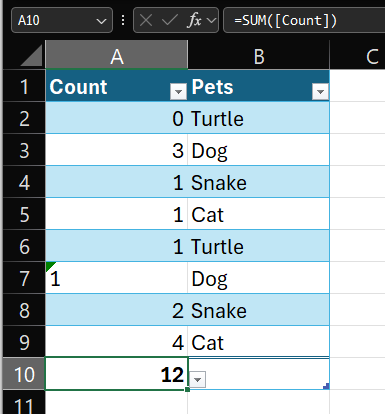
This is an example of type b. The formula is definitely ‘working’ but it isn’t giving us the result that we want.

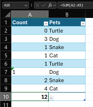
You can see that the function is summing the numbers in column a (or Count). This can also be referenced like =SUM(A2:A9), shown below.

Q2. Does my formula have an obvious error? No, my formula has no errors in it. It has the right number of arguments and no #REF! errors.
Q3. Can Excel answer the question I’m asking?
Does the sheet I’m referencing exist? Yes, I only have one sheet.
Does the table I’m referencing exist? Yes, my table exists at A1:B10
Does the cell I’m referencing have data? Yes.
Count or A1:A5 = number values but one of them appears different….
And there’s our problem.

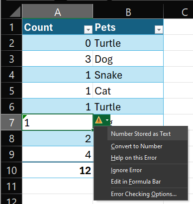
Excel likes to help us out a little with these ones and you can see the little green tag to the left top corner of the cell and the yellow error symbol on the right. Clicking on that displays the pop-out menu above and identifies the potential issue: Number Stored as Text. Because the number is stored as a text value, it cannot be processed as a numerical value by the sum function – or any other function for that matter.
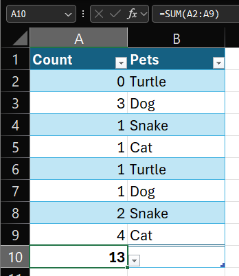
Clicking Convert to Number in this menu will change the data type to a number and your formula will return the correct value.

- An argument is a value, object or variable passed into a function. In most cases the value is being provided to the function to give the function what it needs to complete is purpose. That purpose might be to perform a calculation and return the result or to complete a set task and provide the outcome. ↩︎